4.1. Tutorial 1¶

The following is a basic tutorial about the land cover classification using the Semi-Automatic Classification Plugin (SCP). It is assumed that you have a basic knowledge of QGIS.

Tutorial 1: Your First Land Cover Classification

4.1.1. Tutorial 1: Your First Land Cover Classification ¶

This is a basic tutorial about the use of SCP for the classification of a multispectral image. It is recommended to read the Короткий вступ до дистанційного зондування before this tutorial.

The purpose of the classification is to identify the following land cover classes:

Water;
Built-up;
Vegetation;
Bare soil.

The study area of this tutorial is Greenbelt (Maryland, USA) which is the site of NASA’s Goddard Space Flight Center (the institution that will lead the development of the future Landsat 9 flight segment).

Following the video of this tutorial.

http://www.youtube.com/watch?v=fUZgYxgDjsk

4.1.1.1. Download the Data ¶

We are going to download a Landsat Satellites image (data available from the U.S. Geological Survey) and use the following bands:

Blue;
Green;
Red;
Near-Infrared;
Short Wavelength Infrared 1;
Short Wavelength Infrared 2.

TIP : In case you have a slow connection you can download an image subset from this archive (about 5 MB, data available from the U.S. Geological Survey), unzip the downloaded file, and skip to Convert Data to Surface Reflectance.

Start QGIS and the SCP. Open the tab Download products clicking the button in the Домашня, or in the Меню SCP,

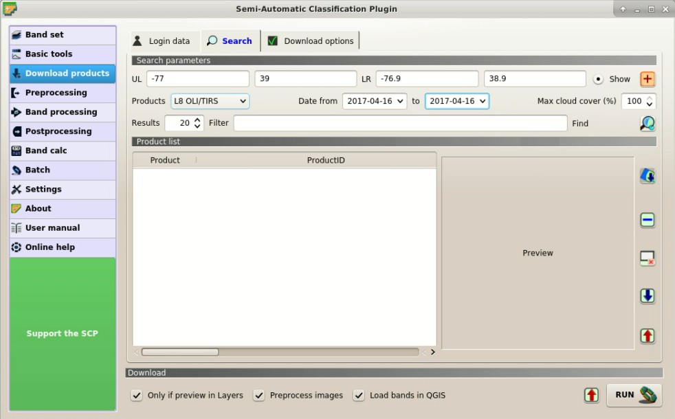
We are searching a specific image acquired on 16 April 2017 because it is cloud free. In Search parameters enter the point coordinates:

UL: -77 / 39
LR: -76.9 / 38.9

TIP : In general it is possible to define the area coordinates clicking the button , then left click in the map for the UL point and right click in the map for the LR point.

Select L8 OLI/TIRS from the Products and set:

Date from: 2017-04-16
to: 2017-04-16

Search products

Now click the button Find and after a few seconds the image will be listed in the Product list. Click the item in the table to display a preview that is useful for assessing the quality of the image and the cloud cover.

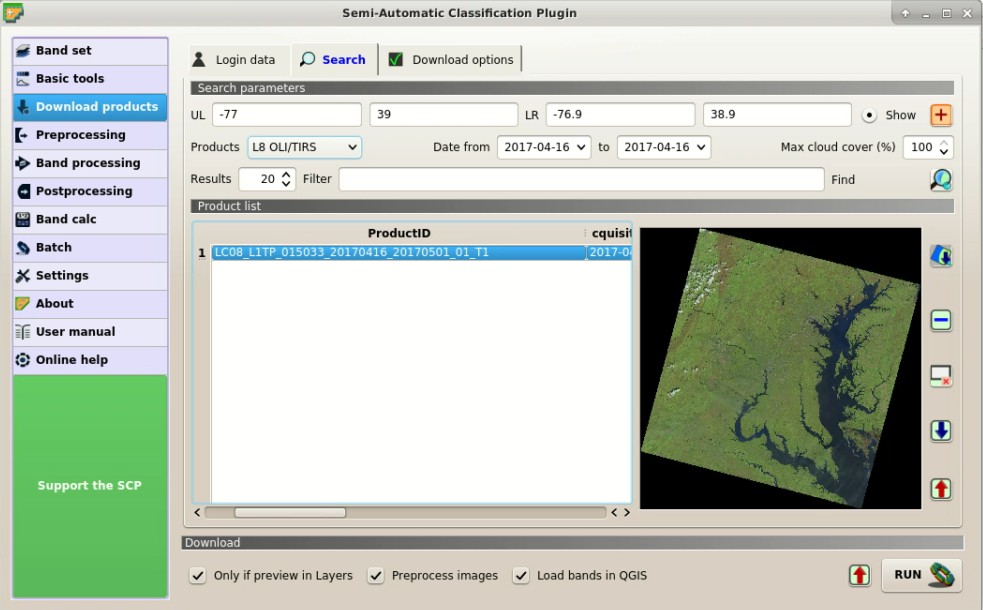
Search result

Now click the button to load the preview in the map.

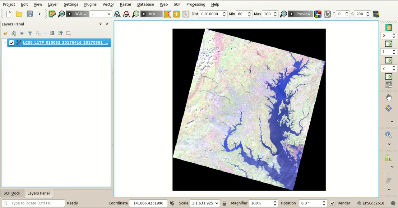
Image preview

We can also select the bands to be downloaded according to our purpose. In particular, select the tab Download options and check only the Landsat bands (that will be used in this tutorial): 2, 3, 4, 5, 6, 7, and the ancillary data.

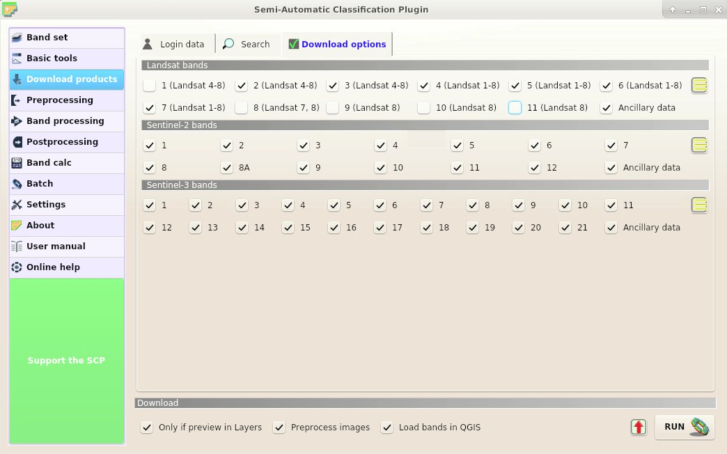
Download options

For the purpose of this tutorial, uncheck the option Preprocess images (you should usually leave this checked) because we are going to preprocess the image in Convert Data to Surface Reflectance. To start the image download, click the button RUN and select a directory where bands are saved. The download could last a few minutes according to your internet connection speed. The download progress is displayed in a bar.

TIP : The option Only if preview in Layers allows for downloading only images in the result table which are loaded as previews in the map. If this option is unchecked, all the products in the list are downloaded.

After the download, all the bands are automatically loaded in the map.

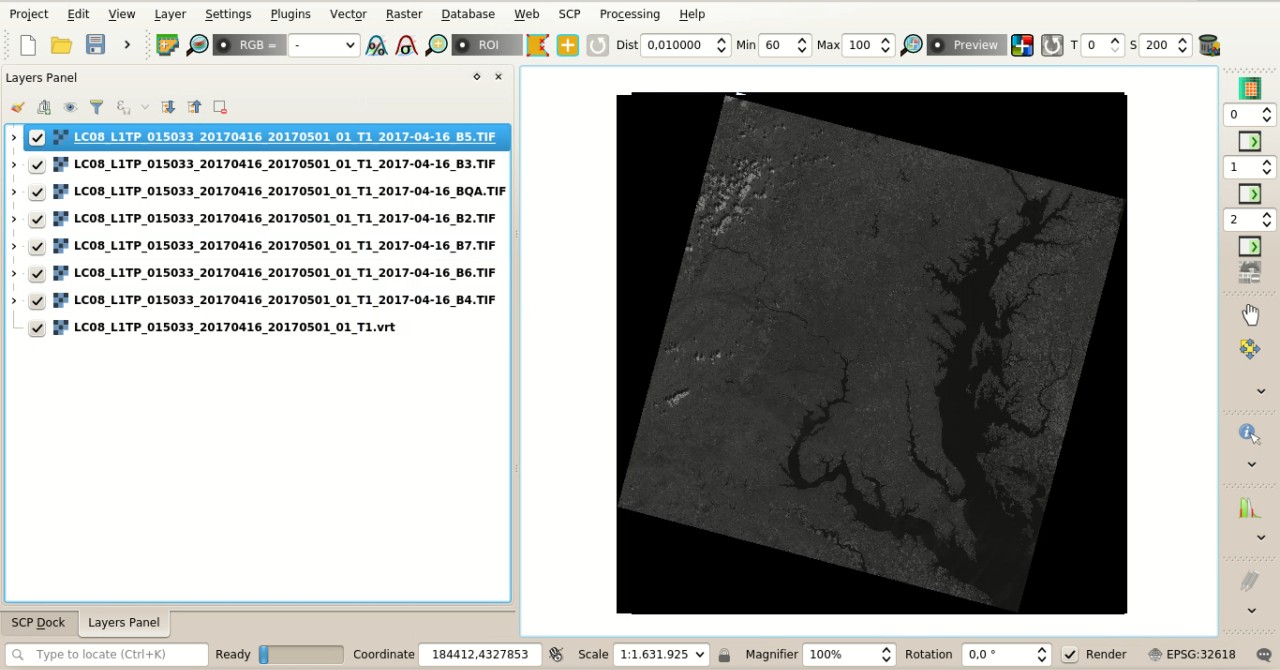
Download of Landsat bands

4.1.1.2. Clip the Data ¶

For for limiting the study area (and reducing the processing time) we can clip the image.

First, we need to define a Band set containing the bands to be clipped. Open the tab Band set clicking the button in the Меню SCP or the Панель SCP.

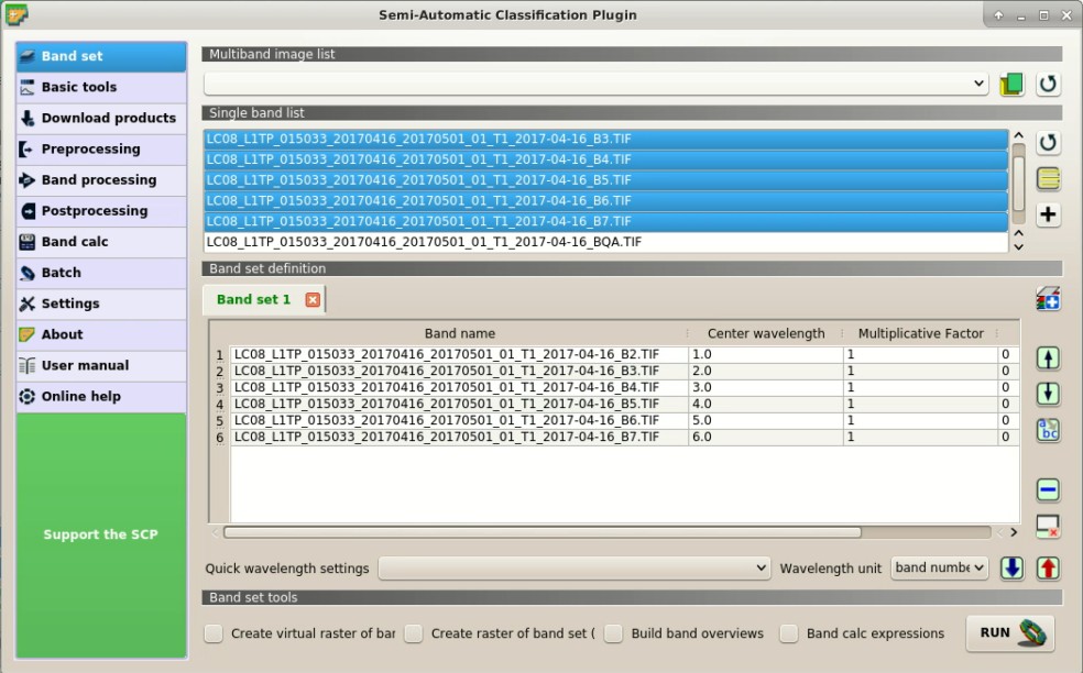
Click the button to refresh the layer list, and select the bands: 2, 3, 4, 5, 6, and 7; then click to add selected rasters to the Band set 1.

Band set for clipping

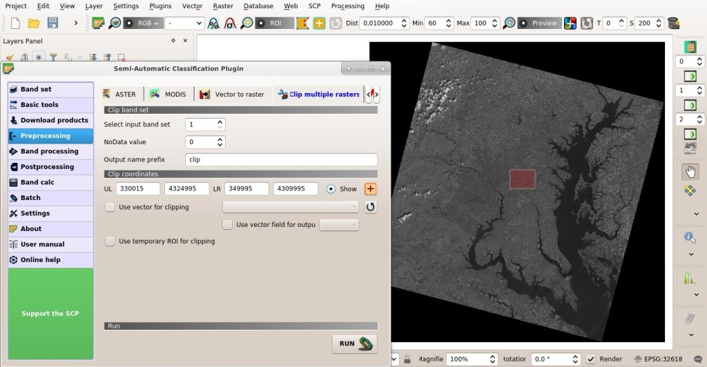
In Preprocessing open the tab Clip multiple rasters. We are going to clip the Band set 1 which contains Landsat bands.

Click the button and select an area such as the following image (left click in the map for the UL point and right click in the map for the LR point), or enter the following values:

UL: 330015 / 4324995
LR: 349995 / 4309995

Clip area

Click the button RUN and select a directory where clipped bands are saved. New files will be created with the file name prefix defined in Output name prefix. When the process is completed, clipped rasters are loaded and displayed.

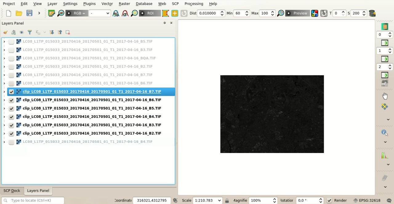
Clipped bands

4.1.1.3. Convert Data to Surface Reflectance ¶

Conversion to reflectance (see Енергетична світність та відбивальна здатність) can be performed automatically. The metadata file (a .txt file whose name contains MTL) downloaded with the images contains the required information for the conversion. Read Перерахунок знімка у значення відбивальності for information about the Відбивальність на поверхні атмосфери (ТОА) and Відбивальність поверхні.

In order to convert bands to reflectance, open the Preprocessing clicking the button in the Меню SCP or the Панель SCP, and select the tab Landsat.

Click the button Directory containing Landsat bands and select the directory of clipped Landsat bands. The list of bands is automatically loaded in the table Metadata.

Click the button Select MTL file and select the metadata file LC08_L1TP_015033_20170416_20170501_01_T1_MTL.txt from the directory of downloaded Landsat images. Metadata information is added to the table Metadata.

In order to calculate Відбивальність поверхні we are going to apply the Корекція DOS1; therefore, enable the option Apply DOS1 atmospheric correction.

TIP : In general, it is recommended to perform the DOS1 atmospheric correction for the entire image (before clipping the image) in order to improve the calculation of parameters based on the image.

For the purpose of this tutorial, uncheck the option Create Band set and use Band set tools because we are going to define this in the following step Define the Band set and create the Training Input File.

In order to start the conversion process, click the button RUN and select the directory where converted bands are saved.

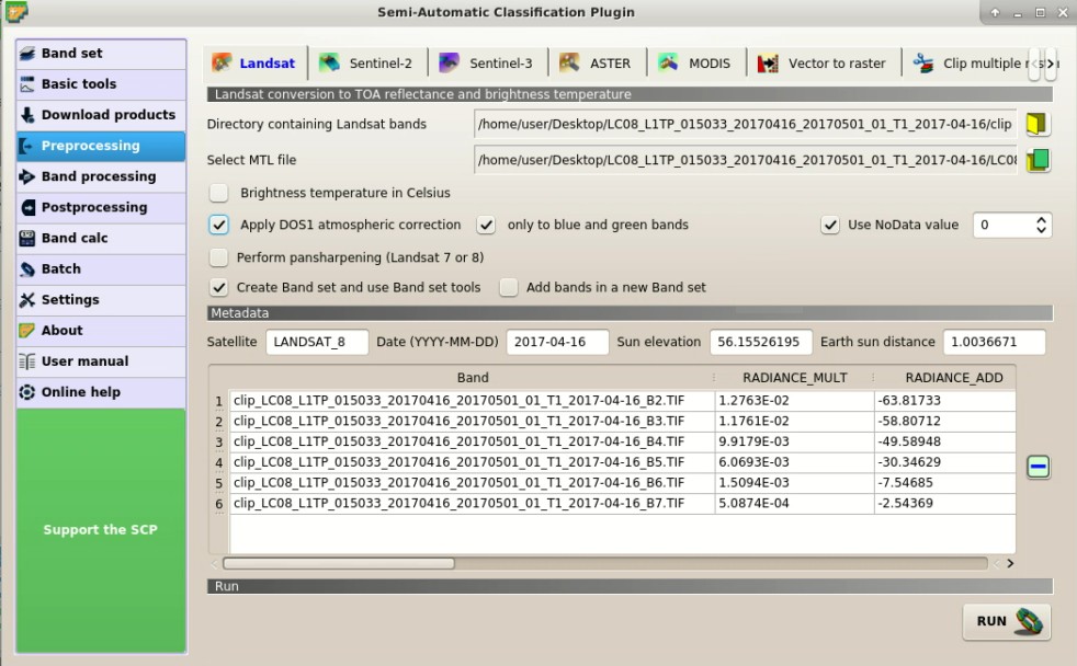
Landsat 8 conversion to reflectance

After a few minutes, converted bands are loaded and displayed (file name beginning with RT_). If Play sound when finished is checked in Classification process settings, a sound is played when the process is finished.

We can remove all the bands loaded in QGIS layers except the ones whose name begin with RT_.

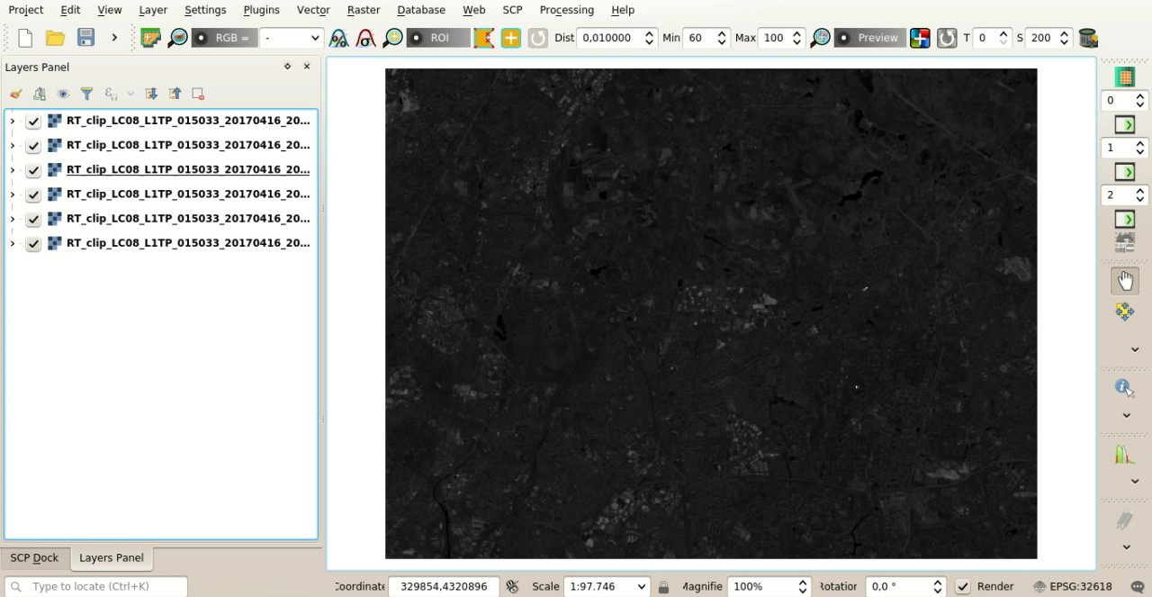
Converted Landsat 8 bands

4.1.1.4. Define the Band set and create the Training Input File ¶

Now we need to define the Band set which is the input image for SCP. Open the tab Band set clicking the button in the Меню SCP or the Панель SCP.

In Band set definition click the button to clear all the bands from active band set created during the previous steps.

Click the button to refresh the layer list, and select all the converted bands; then click to add selected rasters to the Band set.

In the table Band set definition order the band names in ascending order (click to sort bands by name automatically). Finally, select Landsat 8 OLI from the list Quick wavelength settings, in order to set automatically the Center wavelength of each band and the Wavelength unit (required for spectral signature calculation).

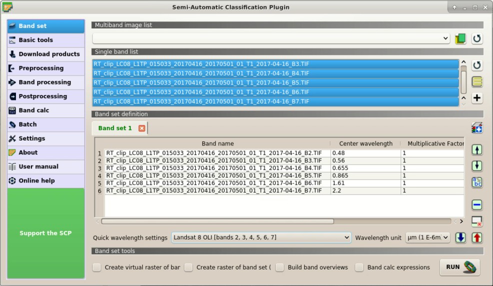
Definition of a band set

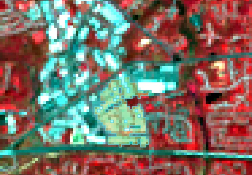
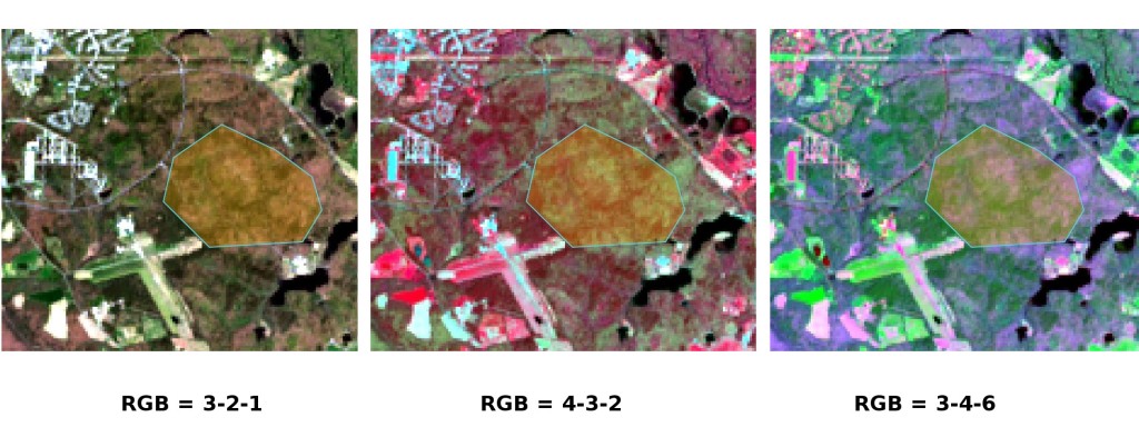
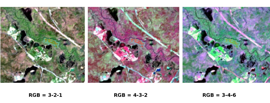
We can display a Кольоровий композит of bands: Near-Infrared, Red, and Green: in the Робоча панель, click the list RGB= and select the item 4-3-2 (corresponding to the band numbers in Band set). You can see that image colors in the map change according to the selected bands, and vegetation is highlighted in red (if the item 3-2-1 was selected, natural colors would be displayed).

TIP : If a Band set is defined, a temporary virtual raster (named Virtual Band Set 1) is created automatically, which allows for the display of Кольоровий композит. In order to speed up the visualization, you can show only the virtual raster and hide all the layers in the QGIS Layers.

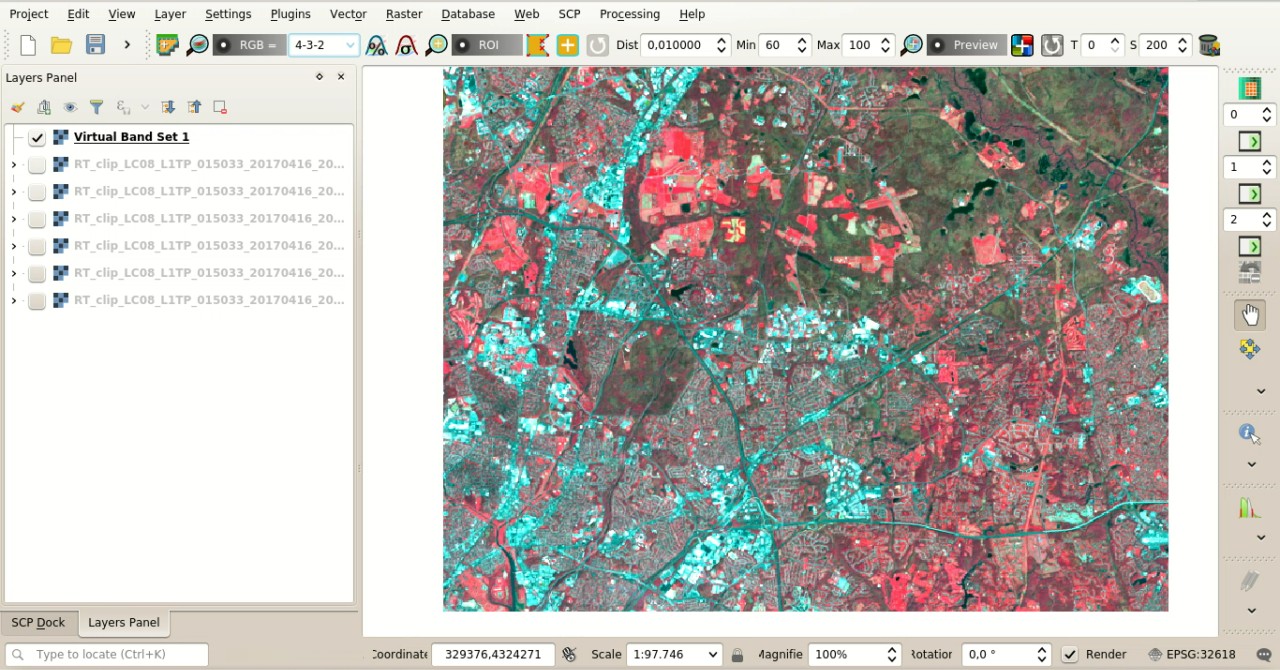
Color composite RGB=4-3-2

Now we need to create the Входові навчальні дані in order to collect Навчальні області (ROIs) and calculate the Спектральна сигнатура thereof (which are used in classification).

In the Панель SCP select the tab Входові навчальні дані and click the button to create the Training input (define a name such as training.scp). The path of the file is displayed and a vector is added to QGIS layers with the same name as the Training input (in order to prevent data loss, you should not edit this layer using QGIS functions).

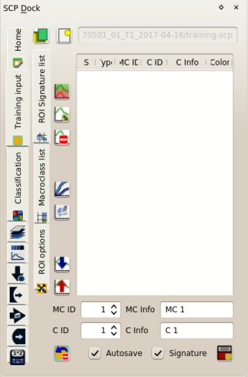
Definition of Training input in SCP

4.1.1.5. Create the ROIs ¶

We are going to create ROIs defining the Класи та макрокласи. Each ROI is identified by a Class ID (i.e. C ID), and each ROI is assigned to a land cover class through a Macroclass ID (i.e. MC ID).

Macroclasses are composed of several materials having different spectral signatures; in order to achieve good classification results we should separate spectral signatures of different materials, even if belonging to the same macroclass. Thus, we are going to create several ROIs for each macroclass (setting the same MC ID, but assigning a different C ID to every ROI).

We are going to used the Macroclass IDs defined in the following table.

Macroclasses

Macroclass name	Macroclass ID
Water	1
Built-up	2
Vegetation	3
Bare soil (low vegetation)	4

ROIs can be created by manually drawing a polygon or with an automatic region growing algorithm.

Zoom in the map over the dark area in the upper right corner of the image which is a water body. In order to create manually a ROI inside the dark area, click the button in the Робоча панель. Left click on the map to define the ROI vertices and right click to define the last vertex closing the polygon. An orange semi-transparent polygon is displayed over the image, which is a temporary polygon (i.e. it is not saved in the Training input).

TIP : You can draw temporary polygons (the previous one will be overridden) until the shape covers the intended area.

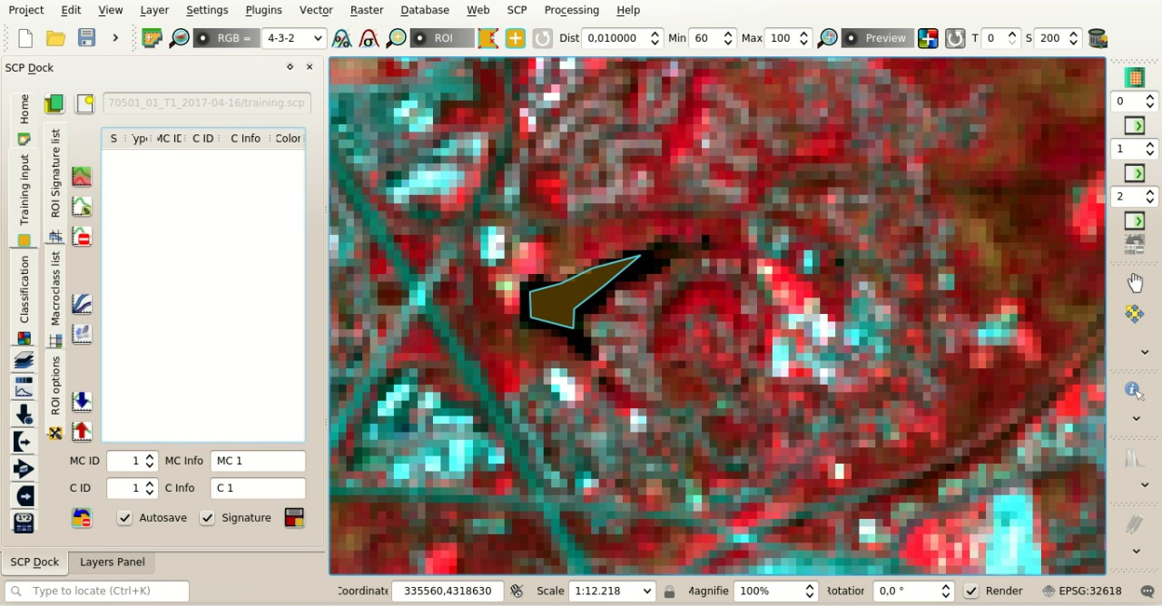
A temporary ROI created manually

If the shape of the temporary polygon is good we can save it to the Training input.

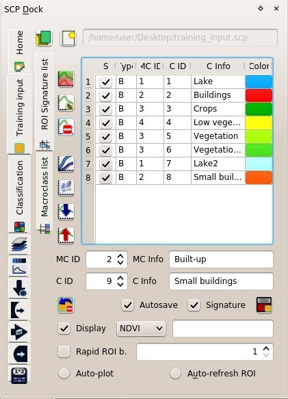
Open the Входові навчальні дані to define the Класи та макрокласи . In the Перелік сигнатур ROI set MC ID = 1 and MC Info = Water; also set C ID = 1 and C Info = Lake. Now click to save the ROI in the Training input.

After a few seconds, the ROI is listed in the Перелік сигнатур ROI and the spectral signature is calculated (because Signature was checked).

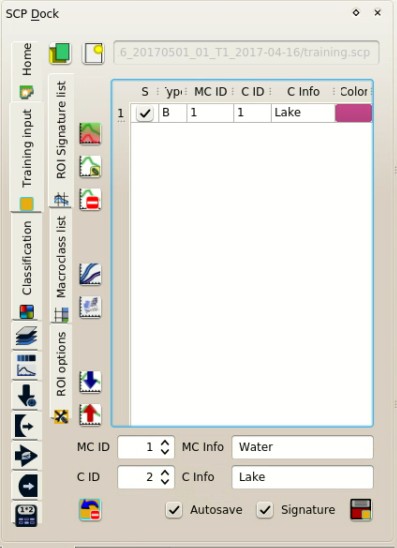
The ROI saved in the Training input

As you can see, the C ID in Перелік сигнатур ROI is automatically increased by 1. Saved ROI is displayed as a dark polygon in the map and the temporary ROI is removed. Also, in the Перелік сигнатур ROI you can notice that the Type is B, meaning that the ROI spectral signature was calculated and saved in the Training input.

You can also see in the tab Макрокласи that the first macroclass has been added to the table Macroclasses .

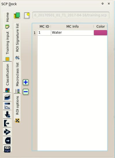
Macroclasses

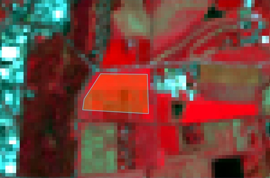
Now we are going to create a second ROI for the built-up class using the automatic region growing algorithm. Zoom in the lower region of the image. In Робоча панель set the Dist value to 0.08 . Click the button in the Робоча панель and click over the purple area of the map. After a while the orange semi-transparent polygon is displayed over the image.

TIP : Dist value should be set according to the range of pixel values; in general, increasing this value creates larger ROIs.

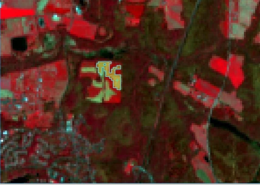
A temporary ROI created with the automatic region growing algorithm

In the Перелік сигнатур ROI set MC ID = 2 and MC Info = Built-up ; also set C ID = 2 (it should be already set) and C Info = Buildings.

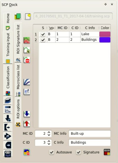
The ROI saved in the Training input

Again, the C ID in Перелік сигнатур ROI is automatically increased by 1.

After clicking the button in the Робоча панель you should notice that the cursor in the map displays a value changing over the image. This is the NDVI value of the pixel beneath the cursor (NDVI is displayed because the function Display is checked in Входові навчальні дані). The NDVI value can be useful for identifying spectrally pure pixels, in fact vegetation has higher NDVI values than soil.

For instance, move the mouse over a vegetation area and left click to create a ROI when you see a local maximum value. This way, the created ROI and the spectral signature thereof will be particularly representative of healthy vegetation.

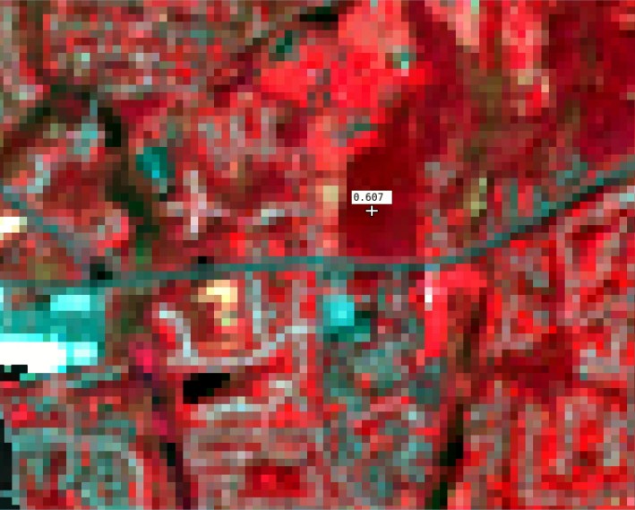
NDVI value of vegetation pixel displayed in the map. Color composite RGB = 4-3-2

Create a ROI for the class Vegetation (red pixels in color composite RGB=4-3-2) and a ROI for the class Bare soil (low vegetation) (green pixels in color composite RGB=4-3-2) following the same steps described previously. The following images show a few examples of these classes identified in the map.

Vegetation. Color composite RGB = 4-3-2

Bare soil (low vegetation). Color composite RGB = 4-3-2

4.1.1.6. Assess the Spectral Signatures ¶

Spectral signatures are used by Алгоритми класифікації for labelling image pixels. Different materials may have similar spectral signatures (especially considering multispectral images) such as built-up and soil. If spectral signatures used for classification are too similar, pixels could be misclassified because the algorithm is unable to discriminate correctly those signatures. Thus, it is useful to assess the Спектральна відстань of signatures to find similar spectral signatures that must be removed. Of course the concept of distance vary according to the algorithm used for classification.

One can simply assess spectral signature similarity by displaying a signature plot. In order to display the signature plot, in the Перелік сигнатур ROI highlight two or more spectral signatures (with click in the table), then click the button . The Графік спектральних сигнатур is displayed in a new window. Move and zoom inside the Графік to see if signatures are similar (i.e. very close). Double click the color in the Відобразити Перелік сигнатур to change the line color in the plot.

We can see in the following figure a signature plot of different materials.

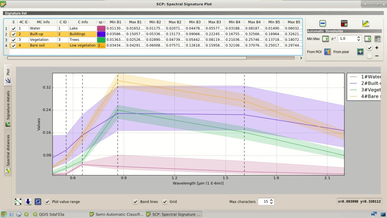
Spectral plot

In the plot we can see the line of each signature (with the color defined in the Перелік сигнатур ROI), and the spectral range (minimum and maximum) of each band (i.e. the semi-transparent area colored like the signature line). The larger is the semi-transparent area of a signature, the higher is the standard deviation, and therefore the heterogeneity of pixels that composed that signature. Spectral similarity between spectral signatures is highlighted in orange in the Відобразити Перелік сигнатур.

Additionally, we can calculate the spectral distances of signatures (for more information see Спектральна відстань). Highlight two or more spectral signatures with click in the table Відобразити Перелік сигнатур, then click the button ; distances will be calculated for each pair of signatures. Now open the tab Спектральні відстані; we can notice that similarity between signatures vary according to considered algorithm.

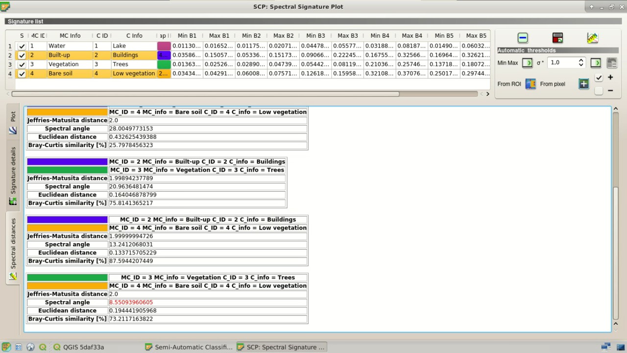
Spectral distances

For instance, two signatures can be very similar for Картографування спектрального кута (very low Спектральний кут), but quite distant for the Максимальної вірогідності (Відстань Джефріса-Мацусіти value near 2). The similarity of signatures is affected by the similarity of materials (in relation to the number of spectral bands available); also, the way we create ROIs influences the signatures.

Spectral signature values, standard deviation and other details such as the number of ROI pixels are displayed in the Характеристика сигнатур.

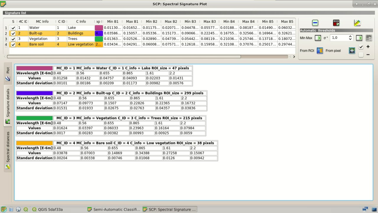
Spectral signature values

We need to create several ROIs (i.e. spectral signatures) for each macroclass (repeating the steps in Create the ROIs), assigning a unique C ID to each spectral signature, and assess the spectral distance thereof in order to avoid the overlap of spectral signatures belonging to different macroclasses.

In the list RGB= of the Робоча панель type 3-4-6 (you can also use the tool RGB list). Using this color composite, urban areas are purple and vegetation is green. You can notice that this color composite RGB = 3-4-6 highlights roads more than natural color (RGB = 3-2-1).

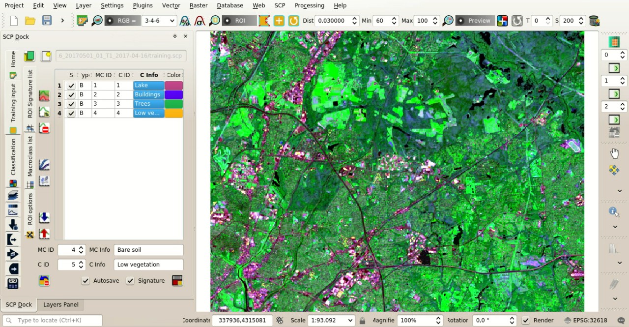
Color composite RGB = 3-4-6

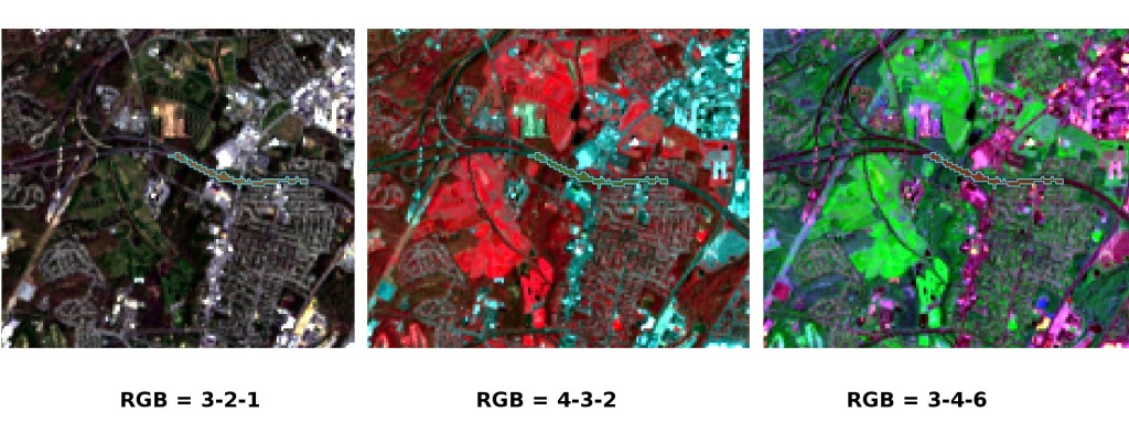
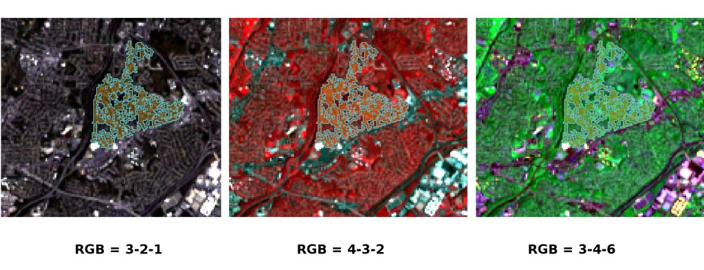
The following examples display a few RGB color composites of Landsat images.

TIP : Change frequently the Кольоровий композит in order to clearly identify the materials at the ground; use the mouse wheel on the list RGB= of the Робоча панель for changing the color composite rapidly; also use the buttons and for better displaying the Input image (i.e. image stretching).

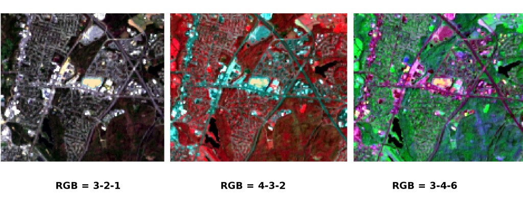
Built-up ROI: large buildings

Built-up ROI: road

Built-up ROI: buildings, narrow roads

Vegetation ROI: deciduous trees

Vegetation ROI: riparian vegetation

It is worth mentioning that you can show or hide the temporary ROI clicking the button ROI in Робоча панель.

TIP : Install the plugin QuickMapServices in QGIS, and add a map (e.g. OpenStreetMap) in order to facilitate the identification of ROIs using high resolution data.

4.1.1.7. Create a Classification Preview ¶

The classification process is based on collected ROIs (and spectral signatures thereof). It is useful to create a Попередній перегляд результатів класифікації in order to assess the results (influenced by spectral signatures) before the final classification. In case the results are not good, we can collect more ROIs to better classify land cover.

Before running a classification (or a preview), set the color of land cover classes that will be displayed in the classification raster. In the Перелік сигнатур ROI, double click the color (in the column Color) of each ROI to choose a representative color of each class.

Definition of class colors

Also, we need to set the color for macroclasses in table Макрокласи.

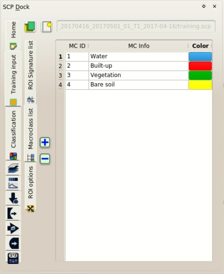
Definition of macroclass colors

Now we need to select the classification algorithm. In this tutorial we are going to use the Максимальної вірогідності.

Open the Класифікація to set the use of classes or macroclasses. Check Use C ID and in Алгоритм select the Maximum Likelihood.

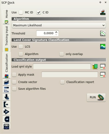
Setting the algorithm and using C ID

In Попередній перегляд результатів класифікації set Size = 300; click the button and then left click a point of the image in the map. The classification process should be rapid, and the result is a classified square centered in clicked point.

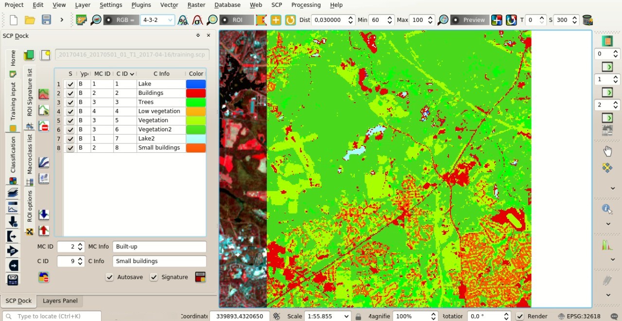
Classification preview displayed over the image using C ID

Previews are temporary rasters (deleted after QGIS is closed) placed in a group named Class_temp_group in the QGIS panel Layers. Now in Класифікація check Use MC ID and click the button in Попередній перегляд результатів класифікації.

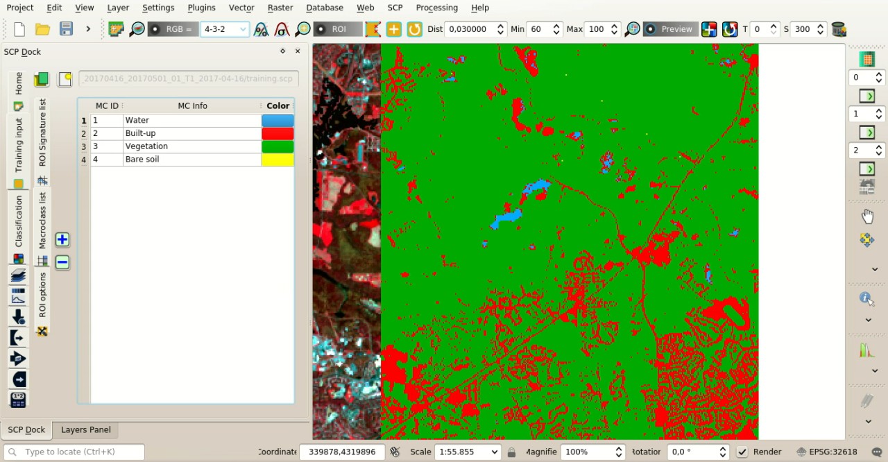
Classification preview displayed over the image using MC ID

We can see that now there are only 4 colors representing the macroclasses.

TIP : When loading a previously saved QGIS project, a message could ask to handle missing layers, which are temporary layers that SCP creates during each session and are deleted afterwards; you can click Cancel and ignore these layers; also, you can delete these temporary layers clicking the button in Робоча панель.

In general, it is good to perform a classification preview every time a ROI (or a spectral signature) is added to the Перелік сигнатур ROI. Therefore, the phases Create the ROIs and Create a Classification Preview should be iterative and concurrent processes.

4.1.1.8. Create the Classification Output ¶

Assuming that the results of classification previews were good (i.e. pixels are assigned to the correct class defined in the Перелік сигнатур ROI), we can perform the actual land cover classification of the whole image.

In Класифікація check Use MC ID. In the Результат класифікації click the button and define the path of the classification output, which is a raster file (.tif). If Play sound when finished is checked in Classification process settings, a sound is played when the process is finished.

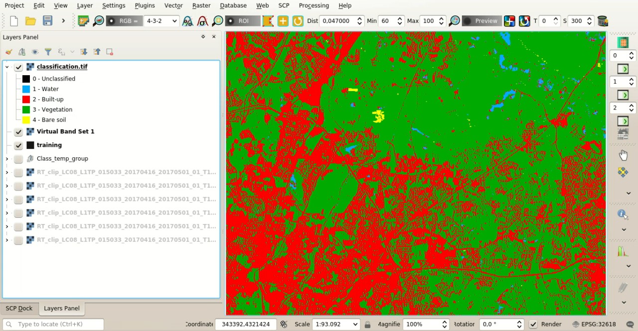
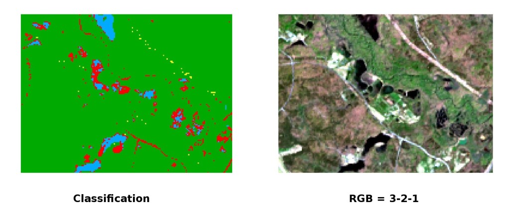
Result of the land cover classification

Well done! You have just performed your first land cover classification.

However, you can see that there are several classification errors, because the number of ROIs (spectral signatures) is insufficient.

Example of error: Water bodies classified as Built-up

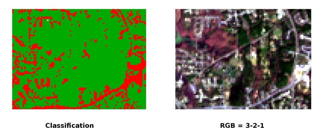
Example of error: Built-up classified as vegetation

We can improve the classification using some of the tools that will be described in other tutorials.